The path is like layers of a video game, where you can’t skip levels.
Table of Contents
Every concept builds on the last. But if you put in real work, not watching some lame ahh YouTube videos about finance, that’s just wasting your time, actual problem-solving work – you can go from knowing nothing to being something in about 18 months.
Forget everything you think you know about trading.
Most people think quantitative trading is about picking stocks. Having opinions on Tesla. Predicting earnings.
Quant trading is about math.
You are mostly working with statistical relationships, pricing inefficiencies, and structural edges that exist because markets are complex systems run by humans who make systematic errors.
Part I: Probability is the Language of Uncertainty
Everything in quantitative finance reduces kinda to 1 question:
What are the odds, and are the odds in my favor?
That’s probability. If you don’t understand probability at a deep level, nothing else in this article matters.
Conditional thinking
Most people think in absolutes. Something is true or it isn’t. Quants think in conditionals. Given what I know, how likely is this?
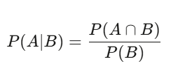
The probability of A given B equals the probability of both happening divided by the probability of B. Profound implications.
A stock goes up 60% of days – that’s the base rate. But on days when volume is above average, it goes up 75% of the time.
That conditional probability is a NOT BS. The raw 60% is NOISY BS.
Bayes’ theorem
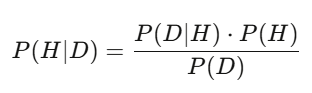
(how likely you’d see this data if your hypothesis were true) * (your prior belief) / (the total probability of seeing this data under any hypothesis).
The denominator sums over all hypotheses.
In practice, you compute this with Monte Carlo sampling.
But the logic is the same. Bayes is how you update your conviction in real time.
A model says a stock should be worth $50. Earnings come out, revenue is 3% above estimate. The Bayesian posterior shifts upward. The traders who update fastest and most accurately win bread.
Expected value and variance your two best friends
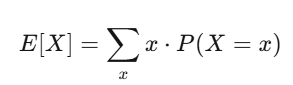
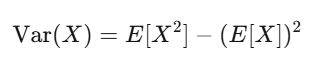
Expected value is your conviction. Variance is your risk.
If your strategy has positive expected value and you can survive the variance, you likely will make money.
Level 1 homework (3-4 weeks at 2 hours/day): 1. Read Blitzstein & Hwang, Introduction to Probability (free PDF from Harvard). Every problem in Chapters 1-6. 2. Code Simulate 10,000 coin flips, verify the law of large numbers visually. 3. Code 2 Implement a Bayesian updater takes a prior and likelihood, returns a posterior.
python
import numpy as np
import matplotlib.pyplot as plt

# Law of large numbers: running average converges to true probability
np.random.seed(42)
flips = np.random.choice([0, 1], size=10000, p=[0.5, 0.5])
running_avg = np.cumsum(flips) / np.arange(1, 10001)

plt.figure(figsize=(10, 4))
plt.plot(running_avg, linewidth=0.7)
plt.axhline(y=0.5, color='r', linestyle='--', label='True probability')
plt.xlabel('Number of flips')
plt.ylabel('Running average')
plt.title('Law of Large Numbers in Action')
plt.legend()
plt.savefig('lln.png', dpi=150)
print(f"After 10,000 flips: {running_avg[-1]:.4f} (true: 0.5000)")
Part II: Statistics
Once you speak probability, you need to learn to listen to data.
That’s statistics and the #1 lesson statistics teaches is “most of what looks like NOT A BS is actually NOISY BS”
Hypothesis testing is the BS detector
You build a model. It backtests at 15% annual return. Is it real?
Set up H_0: “this strategy has zero expected return.” Compute a test statistic. Calculate a p-value – the probability of seeing results this good if H_0 were true.
BUT If you test 1,000 random strategies, 50 of them will show p-values below 0.05 purely by chance.
That’s the multiple comparisons problem. Ur fix is Bonferroni correction divide your significance threshold by the number of tests Or use Benjamini-Hochberg for false discovery rate control.
Every single beginner massively overestimates how much NOT A BS they’ve found. Your first 10 strategies will all be NOISY BS. Accept this now and save yourself a lot of money.
Regression decomposing returns
Linear regression y=Xβ+ϵ is the workhorse. In finance, you regress your strategy’s returns against known risk factors:

The intercept α is your alpha the return that can’t be explained by known factors. If α is zero after accounting for factors, your “edge” is just disguised market exposure.
The OLS estimator:
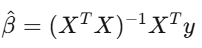
The most important number is α. Use Newey-West standard errors financial data has autocorrelation and heteroskedasticity, so default OLS standard errors are wrong. Using them is like driving with a cracked windshield.
Maximum Likelihood Estimation
Given data x_1,…,x_n, from a model with parameter θ:
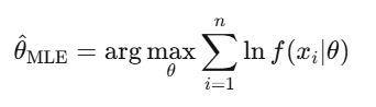
Set the derivative to zero and solve. (or it’s over gng)
MLE is how you calibrate every model in finance fit a GARCH model to volatility, estimate jump-diffusion parameters, calibrate option pricing to market quotes.
It’s asymptotically efficient no other consistent estimator has lower variance for large samples (the Cramér-Rao lower bound).
When someone at a firm says they’re “calibrating” a model, they almost, like always mean MLE.
Level 2 homework (4-5 weeks): 1. Read Wasserman, All of Statistics, Chapters 1-13. 2. Code Download real stock returns with yfinance. Test normality (they’ll fail). Fit a t-distribution via MLE. Compare. 3. Code Run a Fama-French 3-factor regression on a stock portfolio using statsmodels. 4. Code Implement a permutation test shuffle dates 10,000 times, compare shuffled performance to actual.
python
import numpy as np
from scipy import optimize, stats

# Demonstrate fat tails: MLE fit of Student-t to return data
np.random.seed(42)

# Simulate "realistic" returns (fat tails, slight positive drift)
true_df = 4
returns = stats.t.rvs(df=true_df, loc=0.0005, scale=0.015, size=1000)

def neg_log_likelihood(params, data):
    df, loc, scale = params
    if df <= 2 or scale <= 0:
        return 1e10
    return -np.sum(stats.t.logpdf(data, df=df, loc=loc, scale=scale))

result = optimize.minimize(
    neg_log_likelihood, x0=[5, 0, 0.01], args=(returns,),
    method='Nelder-Mead'
)
fitted_df, fitted_loc, fitted_scale = result.x

print(f"MLE degrees of freedom: {fitted_df:.2f} (true: {true_df})")
print(f"MLE location:           {fitted_loc:.6f}")
print(f"MLE scale:              {fitted_scale:.6f}")

# Normality test
_, p_normal = stats.normaltest(returns)
print(f"\nNormality test p-value: {p_normal:.2e}")
print(f"Reject normality? {'YES  fat tails confirmed' if p_normal < 0.05 else 'NO'}")
Part III: Linear Algebra(How To Become Quant)
Linear algebra sounds boring. It’s the machinery that runs everything: portfolio construction, PCA, neural networks, covariance estimation, factor models. You cannot be a quant without being fluent in matrices.
(if u skipped Algebra in school school doing that, it’s over)
Thinking in matrices
A covariance matrix Σ captures how every asset moves relative to every other asset. For 500 stocks, Σ is 500×500 with 125,250 unique entries. Portfolio variance collapses to a single expression
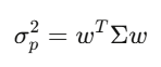
This quadratic form is the core of Markowitz portfolio theory, of risk management, of everything.
Eigenvalues is what actually matters in a universe of stocks
Look at a 500-stock universe and the first 5 eigenvectors explain 70% of all variance. Everything else is NOISY BS.
The first time eigendecomposition u use it the whole world changes. Look at a 500-stock universe and the first 5 eigenvectors explain 70% of all variance. Dimensionality reduction, and it’s the foundation of factor investing.
Level 3 homework (4-6 weeks): 1. Watch Gilbert Strang’s MIT 18.06 lectures all of them. Non-negotiable. 2. Read Strang, Introduction to Linear Algebra. Do the problems. 3. Code PCA decomposition of S&P 500 returns. Plot eigenvalue spectrum. Identify top 3 components. 4. Code Markowitz mean-variance optimization from scratch.
python
import numpy as np
import cvxpy as cp

# ============================================
# Markowitz optimization with cvxpy
# ============================================
np.random.seed(42)
n_assets = 10
mu = np.random.uniform(0.04, 0.15, n_assets)
A = np.random.randn(n_assets, n_assets) * 0.1
cov = A @ A.T + np.eye(n_assets) * 0.01

w = cp.Variable(n_assets)
objective = cp.Minimize(cp.quad_form(w, cov))
constraints = [
    mu @ w >= 0.08,      # minimum return
    cp.sum(w) == 1,       # fully invested
    w >= -0.1,            # max 10% short
    w <= 0.3              # max 30% long
]

prob = cp.Problem(objective, constraints)
prob.solve()

ret = mu @ w.value
vol = np.sqrt(w.value @ cov @ w.value)
sharpe = (ret - 0.03) / vol

print(f"Portfolio return:  {ret:.4f}")
print(f"Portfolio vol:     {vol:.4f}")
print(f"Sharpe ratio:      {sharpe:.4f}")
print(f"Weights: {np.round(w.value, 4)}")
Part IV: Calculus & Optimization
Calculus is the language of change. In finance, everything changes: prices, volatilities, correlations, the entire probability distribution shifts second by second. Calculus describes and exploits those changes.
Derivatives (the math kind): appears in every neural network backpropagation and every Greek calculation.
Taylor expansion:

Delta hedging is the first-order approximation. Gamma hedging adds the second-order correction. And the reason Itô calculus differs from ordinary calculus is precisely because the second-order Taylor term doesn’t vanish for random processes. Just Remember it
Level 4 homework (4-5 weeks): 1. Read Boyd & Vandenberghe, Convex Optimization (free PDF from Stanford), Chapters 1-5. 2. Code Implement gradient descent from scratch. Minimize the Rosenbrock function. 3. Code Solve a portfolio optimization problem with cvxpy including transaction cost constraints.
Part V: Stochastic Calculus
Before stochastic calculus, you’re a data scientist who likes finance.
After it, you’re a quant. QUANTATIVE FINANCE EXPERT, you heard?
This is where you learn to model randomness in continuous time, derive the Black-Scholes equation from first principles, and understand why the trillion-dollar derivatives market works the way it does.
Brownian motion pure randomness, formalized
A Brownian motion (Wiener process) W_t is a continuous-time random walk:
- W_0 = 0
- Increments W_t – W_s ~ N(0, t – s) for t > s
- Non-overlapping increments are independent
- Paths are continuous but nowhere differentiable
The critical insight that everything else depends on: dW_t has “size” dt, which means (dW_t)^2 = dt. This sounds like a technicality, but its the single most important fact in quantitative finance.
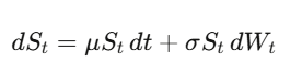
Geometric Brownian Motion models stock prices:

In normal calculus, df = f'(x)dx. You Taylor-expand, and the (dx)^2 term is infinitesimally small you drop it.
But when x is a stochastic process, (dW_t)^2 = dt is first order. You can’t drop it.
Itô’s lemma:
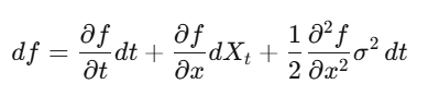
Apply it to an option price and you get Black-Scholes. Formula is the engine behind the entire derivatives industry.
Deriving Black-Scholes from scratch
Follow along with pen and paper.
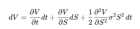
Step 1: Let V(S,t) be an option price. Apply Itô’s lemma:
Step 2: Construct a delta-hedged portfolio Π=V−∂S/∂V⋅S. Compute dΠ:
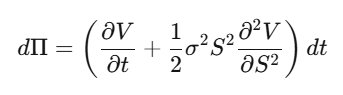
The dW_t terms cancel perfectly. The portfolio is locally riskless.
Step 3: A riskless portfolio must earn the risk-free rate: dΠ=rΠ dtd\Pi = r\Pi \, dt dΠ=rΠdt.
Step 4: Substitute and rearrange:
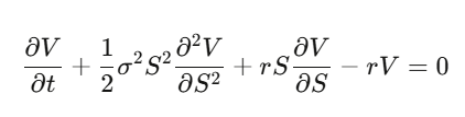
This is the Black-Scholes PDE.
Notice what happened – the drift μ vanished. The option price doesn’t depend on the expected return of the stock. Risk preferences don’t matter. You can price options as if everyone is risk-neutral. The first time this sinks in genuinely mind-bending.
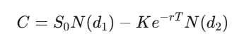
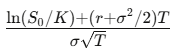
Solving this PDE for a European call with strike K and expiry T gives:
The Greeks
- Delta Δ is How much the option moves per $1 stock move. Your hedge ratio.
- Gamma Γ: How fast delta changes. Your convexity exposure.
- Theta Θ: Time decay. Typically negative for long options.
- Vega V: Sensitivity to volatility. Where most derivatives money is made.
- Rho ρ: Sensitivity to interest rates.
Delta tells you your hedge ratio. Gamma tells you how often to re-hedge. Theta is the cost of holding. Vega is the bread and butter of vol trading desks.
Level 5 homework (6-8 weeks – the hardest level): 1. Read Shreve, Stochastic Calculus for Finance II. The gold standard. 2. Alternative Arguin, A First Course in Stochastic Calculus (newer, more accessible). 3. Derive Apply Itô’s lemma to f(S)=ln(S) where S follows GBM. Get the −σ^2/2. 4. Derive The full Black-Scholes equation from the delta-hedging argument. 5. Code Black-Scholes from scratch. Compare to Monte Carlo. Verify convergence.
python
import numpy as np
from scipy.stats import norm
def black_scholes(S, K, T, r, sigma, option_type='call'):
d1 = (np.log(S/K) + (r + sigma**2/2)*T) / (sigma*np.sqrt(T))
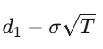
d2 = d1 - sigma*np.sqrt(T)
if option_type == 'call':
return S*norm.cdf(d1) - K*np.exp(-r*T)*norm.cdf(d2)
else:
return K*np.exp(-r*T)*norm.cdf(-d2) - S*norm.cdf(-d1)
def monte_carlo_option(S0, K, T, r, sigma, n_sims=500_000):
"""Price via risk-neutral simulation (drift = r, not mu)"""
Z = np.random.standard_normal(n_sims)
ST = S0 * np.exp((r - sigma**2/2)*T + sigma*np.sqrt(T)*Z)
payoffs = np.maximum(ST - K, 0)
price = np.exp(-r*T) * np.mean(payoffs)
stderr = np.exp(-r*T) * np.std(payoffs) / np.sqrt(n_sims)
return price, stderr
def greeks(S, K, T, r, sigma):
d1 = (np.log(S/K) + (r + sigma**2/2)*T) / (sigma*np.sqrt(T))
d2 = d1 - sigma*np.sqrt(T)
return {
'delta': norm.cdf(d1),
'gamma': norm.pdf(d1) / (S * sigma * np.sqrt(T)),
'theta': -(S*norm.pdf(d1)*sigma)/(2*np.sqrt(T)) - r*K*np.exp(-r*T)*norm.cdf(d2),
'vega': S * np.sqrt(T) * norm.pdf(d1),
'rho': K * T * np.exp(-r*T) * norm.cdf(d2),
}
# Verify: Monte Carlo converges to Black-Scholes
S, K, T, r, sigma = 100, 105, 1.0, 0.05, 0.2
bs = black_scholes(S, K, T, r, sigma)
mc, err = monte_carlo_option(S, K, T, r, sigma)
g = greeks(S, K, T, r, sigma)
print(f"Black-Scholes: ${bs:.4f}")
print(f"Monte Carlo: ${mc:.4f} ± {err:.4f}")
print(f"Difference: ${abs(bs - mc):.4f}\n")
for name, val in g.items():
print(f" {name:>6}: {val:.6f}")Polymarket
This is the most interesting market in the world right now and the math behind it connects everything in this article: probability, information theory, convex optimization, integer programming
How LMSR prices beliefs
The Logarithmic Market Scoring Rule (LMSR), invented by Robin Hanson, powers automated prediction markets. The cost function for n outcomes:
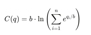
where q_i tracks outstanding shares of outcome i and b is the liquidity parameter. The price of outcome i:
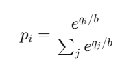
That’s the softmax function – function powering every neural network classifier.
Prices always sum to 1, always lie in (0,1), and always exist providing infinite liquidity. The market maker’s maximum loss is bounded at b * ln(n)
The Quant Career Landscape
4 archetypes: Quant Researcher The most-cracked guy who finds patterns in petabytes, builds predictive models, designs strategies. Needs PhD-level math/stats/ML, or exceptional undergraduate achievement. At firms like Jane Street, QRs work with tens of thousands of GPUs.
Quant Developer/Engineer The mid-cracked guy, mostly the builder. Trading platforms, execution engines, real-time data pipelines. Makes the researcher’s model actually trade. Needs production C++/Rust/Python, low-latency systems.
Quant Trader Either the biggest degen or the most-cracked guy, mostly the decision-maker. Runs capital, manages risk, makes real-time calls. Highest compensation variance – eight figures in exceptional years.
Risk Quant The most-cracked guy or just insanely experienced corporate guy, mostly the guardian. Model validation, VaR, stress testing, regulatory compliance. Steadier career, lower ceiling. The emerging AI/ML Quant role signal generation with deep learning is the fastest-growing, with hiring up 88% year-over-year in 2025.
What it pays:
Level Top Tier (Jane Street, Citadel, HRT) New grad $300K-$500K+ total comp Mid career (3-7yr)$550K-$950K Senior (8+yr)$1M-$3M+ Star trader/PM $3M-$30M+ Mid Tier (Two Sigma, DE Shaw) New grad $250K–$350K Mid career (3-7yr) $350K–$625K Senior (8+yr) $575K–$1.2M Star trader/PM idk
Jane Street’s average employee compensation was reported at $1.4 million/year in H1 2025. That’s the average though
The interview gauntlet
Resume screen -> Online assessment (mental math via Zetamac – target 50+, logic puzzles) -> Phone screen (probability problems, betting games) -> Superday (3-5 back-to-back interviews, mock trading, coding, whiteboard derivations).
Jane Street gives problems intentionally too hard to solve alone – they test how you use hints and collaborate.
Over two-thirds of their recent intern class studied CS; over a third studied math. Finance knowledge generally not required.
The #1 prep resource Xinfeng Zhou’s Green Book (A Practical Guide to Quantitative Finance Interviews) – 200+ real problems. Supplement with
(“LeetCode for quants”) Brainstellar Jane Street’s Figgie card game
The Complete Toolbox
Python stack Data: pandas, polars (Polars is 10-50x faster on large datasets) Numerics: numpy, scipy ML (tabular): xgboost, lightgbm, catboost ML (deep): pytorch Optimization: cvxpy Derivatives: QuantLib (Industry-grade, C++ backend) Stats: statsmodels Backtesting: NautilusTrader Backtesting (simpler): backtrader, vectorbt (Easier starting point) Quant research: Microsoft Qlib (17K+ stars, AI-oriented) RL for trading: FinRL (10K+ stars)
C++ and Rust Tbh i don’t know anything about this. This is what I’ve found: C++ libraries: QuantLib, Eigen, Boost. Rust: RustQuant for option pricing, NautilusTrader as the Rust+Python paradigm (Rust core for speed, Python API for research).
Data sources Free: yfinance, Finnhub (60 calls/min), Alpha Vantage. Mid-range:
($199/mo, sub-20ms latency), Tiingo. Enterprise: Bloomberg Terminal (~$32K/yr), Refinitiv, FactSet. Blockchain: Alchemy (free tier with archive access).
Solvers Gurobi: Fastest commercial MIP solver, free academic license. Essential for combinatorial arbitrage. Google OR-Tools: Strongest free solver. PuLP/Pyomo: Python modeling interfaces.
The Reading List (In Order)
Mathematics
- Blitzstein & Hwang – Introduction to Probability (free PDF from Harvard)
- Strang – Introduction to Linear Algebra + MIT 18.06 lectures
- Wasserman – All of Statistics
- Boyd & Vandenberghe – Convex Optimization (free PDF from Stanford)
- Shreve – Stochastic Calculus for Finance I & II
Quant finance
- Hull – Options, Futures, and Other Derivatives
- Natenberg – Option Volatility and Pricing
- López de Prado – Advances in Financial Machine Learning
- Ernest Chan – Quantitative Trading
- Zuckerman – The Man Who Solved the Market
Interview prep
- Zhou – Practical Guide to Quantitative Finance Interviews (Green Book #1)
- Crack –Heard on the Street
- Joshi – Quant Job Interview Questions
Competitions
- Jane Street Kaggle ($100K prize)
- WorldQuant BRAIN (100K+ users, pays for alpha signals)
- Citadel Datathon (fast-track to employment)
- Jane Street monthly puzzles (above interview difficulty)
Three things I wish I’d known earlier
Estimation error is the real enemy. Full Kelly betting, unconstrained Markowitz, ML models with too many features – they all fail for the same reason: overfitting NOISY BS in parameter estimates.
The math works perfectly with true parameters. You never have true parameters. The gap between theory and practice is always estimation error, and the best quants are the ones who respect it.
Tools have democratized. Conviction hasn’t. Anyone can access QuantLib, Polygon.io, and PyTorch. Technology is necessary but not sufficient. Edge lives in unique data, unique models, or unique execution – not better pip installs.
The math is the moat AI can write code and suggest strategies. But the ability to derive why Itô’s lemma has an extra term, to prove that discounted prices are martingales under the risk-neutral measure, to know when a convex relaxation is tight versus loose in a combinatorial market that mathematical fluency separates quants who build edge from quants who borrow it. And borrowed edge expires.
Join for more update and get real-time alerts here: t.me/DailyKoinUpdate
Tags
Quantitative Finance Roadmap,AI ML Quant Salary 2026, QuantFinance, Quant Analyst
You May Also Read:
- SASUF-NRF Seed Grants 2026: Eligibility, Funding, Deadlines and Full Application Guide
- How to Install Claude Code on Ubuntu Linux 2026:The Ultimate Setup Guide for High Velocity AI Engineering
- How I Turned Claude and Obsidian into a Self-Running Business Brain (And You Can Too)
- Best GitHub repos for Claude code that will 10x your next project
- Google Stitch: The Free Tool That Turns Plain English Into Professional App Designs


2 thoughts on “How To Become Quant full Roadmap from zero to pro level guide”