One of the most practical learning resources comes from the MIT Financial Mathematics course available on MIT OpenCourseWare. The lectures cover the same foundations used in hedge funds and algorithmic trading systems.
This guide explains the key concepts from that course and shows how they relate to prediction market trading and Polymarket style markets. No hype, no fake promises, just real mathematics that professionals use every day.
Table of Contents
Why MIT Financial Mathematics Matters for Prediction Markets
Prediction markets convert real world events into probabilities. A contract priced at 0.35 suggests the market believes the event has about a 35 percent chance of happening.
That idea looks simple, yet the machinery behind probability estimation involves serious quantitative tools. MIT teaches these tools through topics such as linear algebra, probability theory, stochastic processes, regression, and portfolio risk management.
Once you understand these concepts, market prices start to look less like numbers and more like probability models.
Phase 1 Linear Algebra and the Hidden Structure of Market Portfolios
Most retail traders ignore linear algebra. Quantitative traders treat it as a core tool.
A matrix often represents data such as price changes across contracts. Imagine tracking daily price moves for dozens of prediction markets. Each row could represent time and each column a contract.
Mathematically a matrix also represents a transformation. It shows how risk moves across a portfolio.
Eigenvalues and Eigenvectors in Market Correlations
The equation Av = λv describes eigenvalues and eigenvectors.
Eigenvectors represent directions where the transformation only scales the vector rather than rotating it. Eigenvalues measure the strength of that scaling.
In portfolio analysis, eigenvectors often reveal hidden risk factors. Researchers commonly use Principal Component Analysis to extract these factors from correlation matrices.
For example, during election cycles many political contracts move together. One dominant factor often drives most of the movement.
This means a trader may hold 100 contracts but actually carry exposure to only a few underlying drivers.
Singular Value Decomposition
Singular Value Decomposition breaks a matrix into components that reveal the number of independent movements in the system.
Quantitative analysts use SVD to detect hidden correlations in financial data. When applied to prediction markets, it often shows that several contracts react to the same underlying news or sentiment shift.
Phase 2 Probability Theory and Distribution Mistakes
Probability theory forms the backbone of quantitative trading.
Many beginners assume financial returns follow a normal distribution. That assumption works in textbooks but fails in many market settings.
Why Log Normal Models Matter(MIT Financial Mathematics Course)
Asset prices cannot drop below zero. Because of this constraint, financial mathematics often models prices using a log normal distribution rather than a standard normal distribution.
This approach treats logarithmic returns as normally distributed while ensuring prices remain positive.
The concept appears in classical financial models such as the Black Scholes framework.
Law of Large Numbers and Trading Edge
The Law of Large Numbers states that the average of many independent trials approaches the expected value.
For traders this means a strategy with a small statistical edge becomes profitable only over many trades.
A single trade proves nothing. Thousands of trades reveal the real performance of a model.
Central Limit Theorem
The Central Limit Theorem explains why aggregated results often appear normally distributed even if individual outcomes do not follow a normal distribution.
This principle helps analysts evaluate the long term behavior of trading strategies.
Phase 3 Stochastic Processes and Price Movement
Financial mathematics models prices using stochastic processes.
A stochastic process describes a sequence of random variables evolving over time. Instead of predicting one outcome, it describes a distribution of possible paths.
Random Walk and Market Uncertainty
One of the simplest models is the random walk.
Each step moves up or down randomly. Over time the uncertainty grows roughly with the square root of time.
This relationship explains why longer time horizons increase uncertainty but not linearly.
Markov Chains and Market Information
Markov models assume that the current state summarizes all available information. Future outcomes depend only on the present state.
Many pricing models rely on this assumption because it simplifies calculations.
However real markets often contain extra signals such as order flow patterns and liquidity changes. Skilled traders look for those signals.
Martingales and Fair Market Prices
A martingale represents a process where the expected future value equals the current value given all known information.
Many financial pricing models use martingale logic under the risk neutral framework.
The implication remains simple. Traders cannot beat a fair market through clever timing alone. Real edge comes from better probability estimates or superior information processing.
Phase 4 Regression Models in Prediction Markets(MIT Financial Mathematics Course)
Serious trading models rely on data. Regression analysis helps connect signals with outcomes.
For prediction markets the outcome usually represents contract resolution. Possible signals include polling data, sentiment indicators, historical base rates, and price momentum.
Ordinary Least Squares Regression
Ordinary Least Squares estimates parameters by minimizing squared differences between predictions and actual results.
The Gauss Markov theorem states that OLS provides the best linear unbiased estimator under certain conditions.
Financial data often violates these assumptions because variance changes over time. Analysts therefore apply weighted regression or more advanced estimators.
Phase 5 Value at Risk and Downside Protection
Professional traders spend as much time on risk management as they spend on return generation.
One widely used measure is Value at Risk, often abbreviated as VaR.
VaR estimates the maximum loss expected over a certain time horizon at a chosen confidence level.
Common VaR Approaches
Financial institutions usually rely on three methods.
Parametric models assume a statistical distribution of returns
Monte Carlo simulation generates thousands of possible scenarios
Historical simulation applies real past movements to current portfolios
Each approach offers strengths and weaknesses. Analysts often combine them to obtain a more robust risk estimate.
Phase 6 Volatility Clustering and GARCH Models
Financial markets show a clear pattern called volatility clustering.
Large price swings tend to follow large swings. Quiet periods often follow quiet periods.
Economist Robert Engle introduced ARCH models to capture this behavior. Later research expanded the framework into GARCH models.
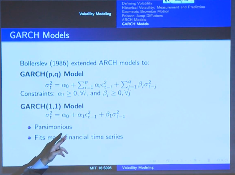
These models estimate future volatility based on past shocks and previous volatility levels.
Traders use them to understand how long uncertainty may remain elevated after major news events.
Phase 7 Portfolio Theory and Efficient Risk Allocation
Modern Portfolio Theory studies how investors balance expected return and risk.
Harry Markowitz introduced the concept of the efficient frontier, which represents the best achievable return for each level of risk.
The Sharpe ratio measures how much return a portfolio produces relative to its volatility.
Many quantitative funds also apply risk parity, where each position contributes equal risk rather than equal capital.
This approach helps control exposure in portfolios containing assets with very different volatility levels.
Phase 8 Factor Models and Hidden Market Drivers(MIT Financial Mathematics Course)
Factor models simplify complex portfolios by identifying a small number of underlying drivers.
A typical model represents returns as a combination of common factors and asset specific noise.
Analysts often estimate these factors using Principal Component Analysis.
In large asset groups, the first few components usually explain most of the total variance.
For prediction markets this may represent broad political sentiment, macro events, or category level trends.
Understanding factor exposure helps traders manage risk more effectively.
Sources
MIT OpenCourseWare Financial Mathematics
Hull Options Futures and Other Derivatives
Engle ARCH Econometrica
Markowitz Portfolio Selection Journal of Finance
Join for more update and get real-time alerts here: t.me/DailyKoinUpdate
Tags
Quant Trading MIT Course, Polymarket Analysis, Financial Mathematics, Risk Management, Predictive Modeling, Linear Algebra, Stochastic Processes, GARCH Volatility, Portfolio Theory, Quantitative Trading Systems
You May Also Read:
- SASUF-NRF Seed Grants 2026: Eligibility, Funding, Deadlines and Full Application Guide
- How to Install Claude Code on Ubuntu Linux 2026:The Ultimate Setup Guide for High Velocity AI Engineering
- How I Turned Claude and Obsidian into a Self-Running Business Brain (And You Can Too)
- Best GitHub repos for Claude code that will 10x your next project
- Google Stitch: The Free Tool That Turns Plain English Into Professional App Designs